Data Preparation

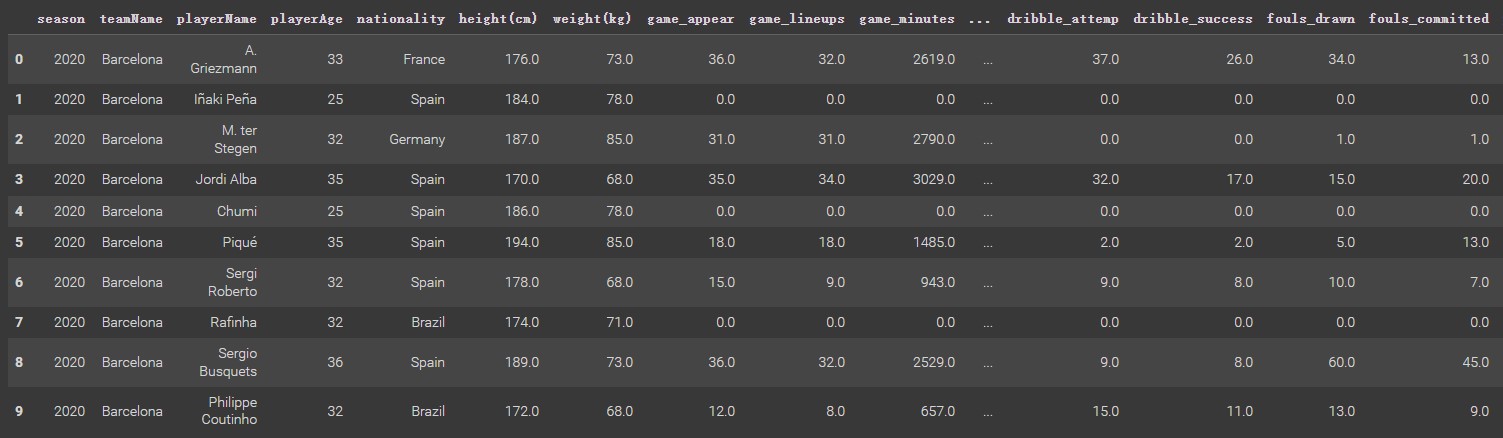
Selecting columns of season, teamName, playerName, position, game_appear, game_lineups, game_minutes. key_pass, pass accuracy, and fouls drawn in the player dataset. Calculating shot success rate by goals_total/shots_total, calculating duel success rate by duel_won/duel_total, and calculating dribble success rate by dribble_success/dribble_attempt. Then, pick players whose position is the attacker and season from 2020 to 2022. There are some NaN values due to some players being transferred by clubs at the beginning of the season, so dropping these NaN values. After that, generate a new data frame.

The Player Dataset

The New Datafram

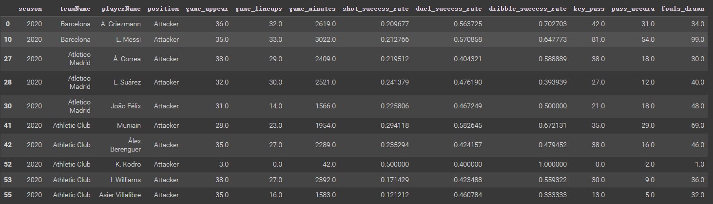
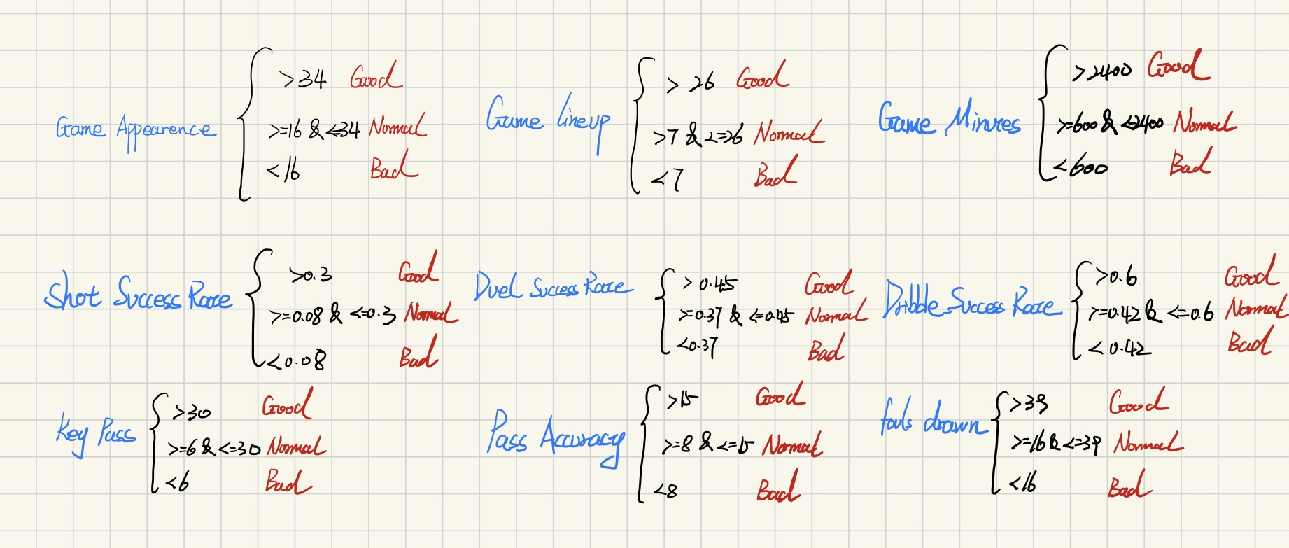
Since this new dataframe does not have a label column, it does not work for using multinomial Naïve Bayes, so it is necessary to add a label column. Data in this dataset is used to predict whether the performance of an attacker is good or not. Thus, the label is divided into three categories: good, normal, and bad. Due to game_appear, game_lineups, game_minutes, key_pass, pass_accuracy, foul_drawn, shot_success_rate, duel_success_rate, and _dirbble_success_rate are numeric variables, so it needs to create labels for all of them (still three categories: good, normal, bad). Finally, these variable labels are aggregated to generate a final label for each row.

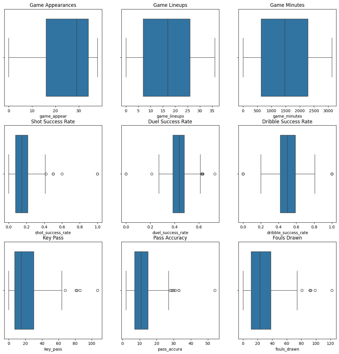
Plot the boxplot of each variable to determine how to divide categories by numeric value, then add a label column for each variable to the dataframe.

The boxplot for each numeric variable

Labels For Each Numeric Variabel

Using the Python code below, count which categories appear the most in each row and serve as the final label. And final dataframe below is

cols = ['game_appear_labels','game_lineups_labels','game_minutes_labels',
        'shot_success_rate_labels','duel_success_rate_labels','dribble_success_rate_labels',
        'key_pass_labels','pass_accura_labels','fouls_drawn_labels']

player['label'] = player[[col for col in cols]].mode(axis=1)[0]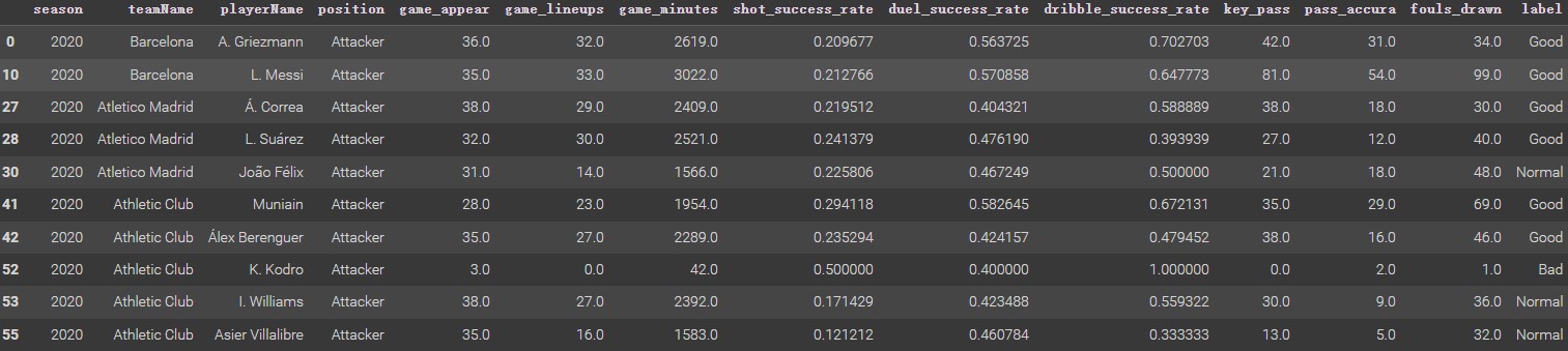

Final DataFrame

Train Dataset and Test Dataset Splitting

import pandas as pd
import numpy as np
import seaborn as sns
import matplotlib.pyplot as plt
from sklearn.model_selection import train_test_split
from sklearn.naive_bayes import MultinomialNB
from sklearn.metrics import confusion_matrix


player = pd.read_csv("label_clean_DF.csv")

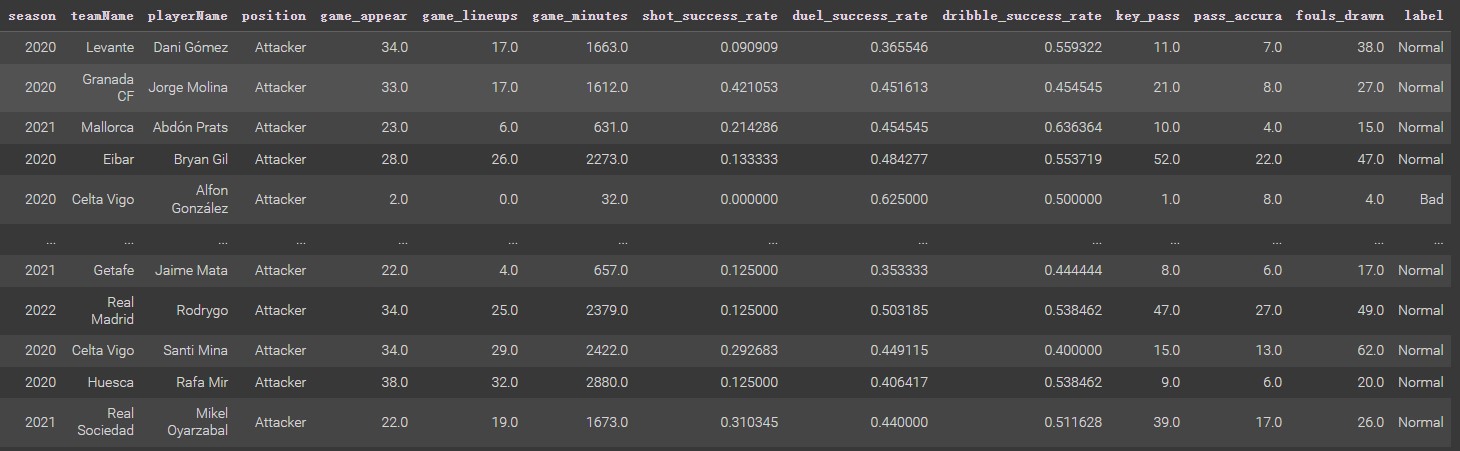
playerTrainDF, playerTestDF = train_test_split(player,test_size = 0.3)
playerTestLabel = playerTestDF['label']

playerTestDF = playerTestDF.drop(["label"],axis = 1)
playerTrainDF_nolabel = playerTrainDF.drop(["label"],axis = 1)
playerTrainLabel = playerTrainDF['label']

dropcols = ['season','teamName','playerName','position']
playerTrainDF_nolabel_quant = playerTrainDF_nolabel.drop(dropcols,axis = 1)
playerTestDF_quant = playerTestDF.drop(dropcols,axis=1)

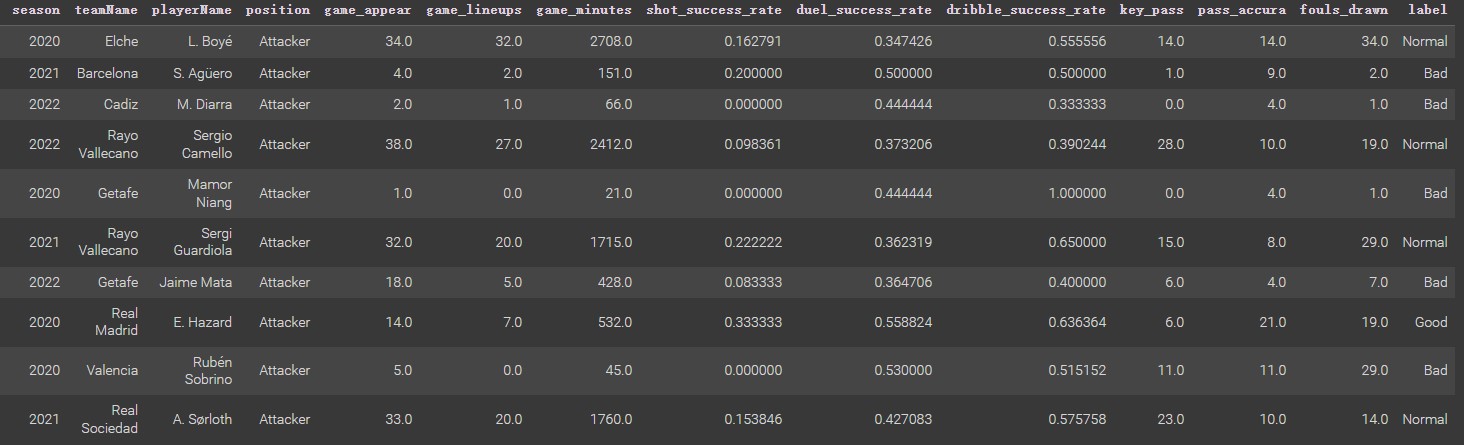
Using the train_test_split function, and getting the train set and test set (shown below). Here the test dataset is divided into 30% of the total dataframe. This allows us to evaluate the generalization ability of the multinomial NB model divided by the final dataframe 70% as the training dataset, and the final dataset 30% as the test dataset, Creating a disjoint split is essential for the prediction model. If there are overlapping samples in the training set and test dataset, the model will view the labels in the test set and remember them during training. It can lead to errors in the evaluation of the performance of the model. Just as a student knows the answers to an exam in advance, a teacher cannot determine whether this student has really learned content by the test score.