Accuracy of Model’s Prediction
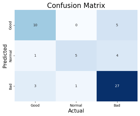
The prediction results are shown through the following the confusion matrix and line plot. The confusion matrix can evaluate the prediction performance of this multinomial Naive Bayes model. First of all, it can calculate the accuracy of the model through this matrix. According to the formula of accuracy:
$$ \frac{\text{Number of corretly classified Samples}}{\text{Total Number of Sampels}} = \frac{10+5+27}{10+0+5+1+5+4+3+1+27} = \frac{42}{56} \approx 0.75$$
The accuracy of the model’s prediction is 75%. This result is the same as the result of accuracy_score in the Sklearn library.
from sklearn.metrics import accuracy_score
accuracy = accuracy_score(playerTestLabel, prediction)
print(accuracy)

>>> 0.75
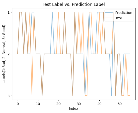
The line plot also reveals that roughly 35% of the folds in the plot are not overlapped. The 75% correct accuracy of prediction may indicate that the predictive ability of this model is at intermediate to upper intermediate level. Thus, the predicted results that can be convincing.
Not only that, getting the precision rate for each category by using the confusion matrix:
$$\text{‘Good’ Precision} = \frac{10}{10+1+3} = \frac{10}{14} \approx 0.71$$
$$\text{‘Normal’ Precision} = \frac{5}{0+5+1} = \frac{5}{6} \approx 0.83$$
$$\text{‘Bad’ Precision} = \frac{24}{5+4+27} = \frac{24}{36} \approx 0.75$$
According to the these formulas can be seen that the category of Nomral has highest precision rate, which is about 83%. The next highest precision rate for the category of Bad is about 75%. The category of Good has a precision rate of about 71%. Therefore, predicting the category as Normal is the most accurate, and predicting the category as Good is less effective than the other two categories.
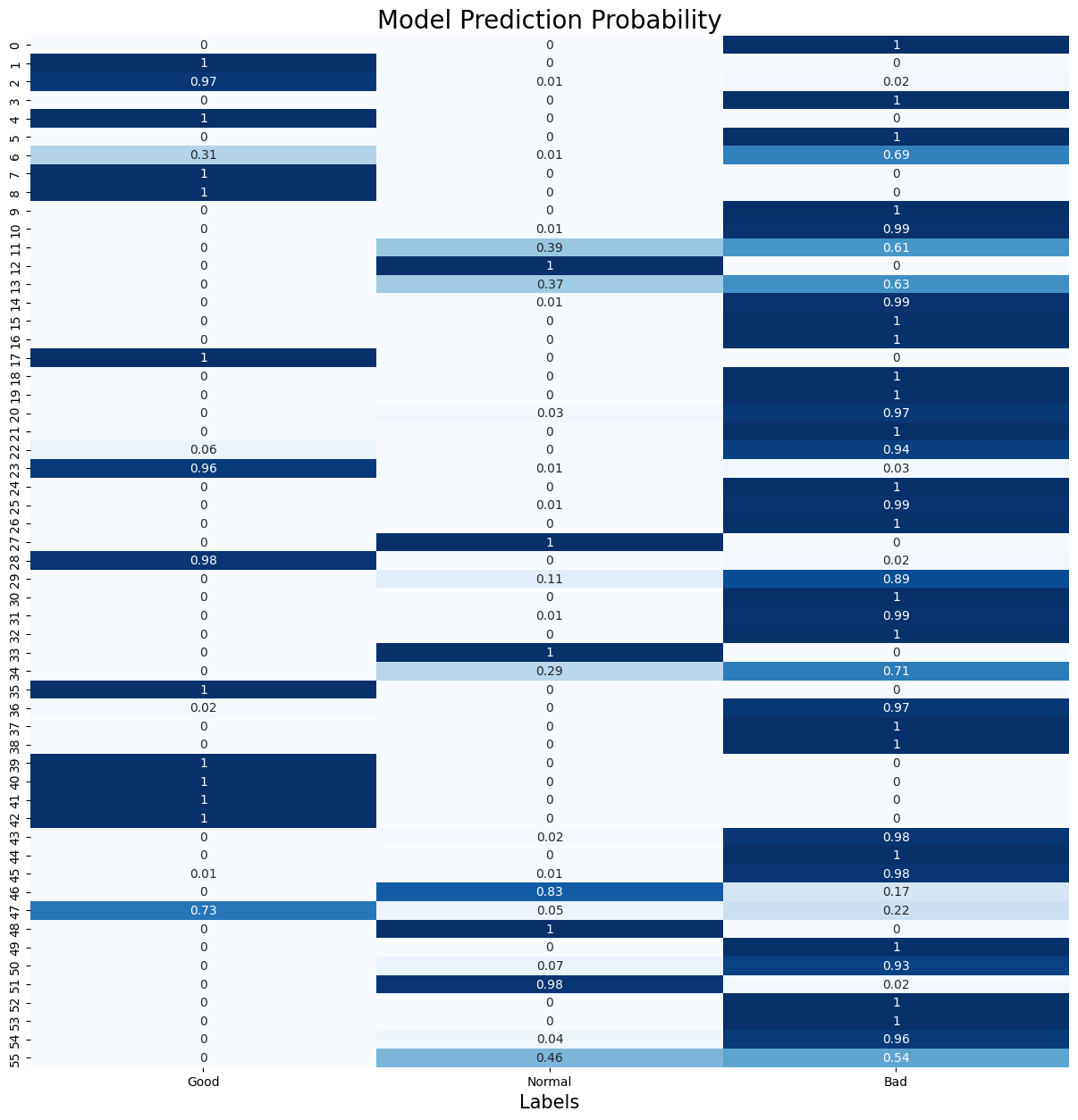
From the following model prediction probability, if there is a situation like Good = 0.33, Normal = 0.33, Bad = 0.34 or Good = 0.47, Normal = 0.48, Bad = 0.05. It indicates that the model has high uncertainty when classifying samples. In this case, the model fails to clearly determine which categories the sample belongs to and distribute the probabilities across multiple categories. However, this model does not appear in this situation which shows that the classification accuracy is still acceptable.
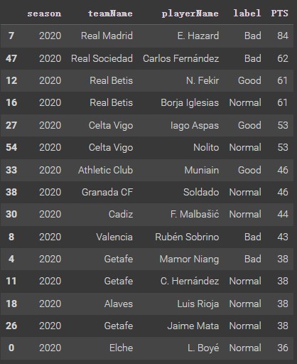
The following is a part of the predicted dataset. The model’s predictions are good. For example, Real Madrid attacker Hazard. He is a player that Real Madrid bought from Chelsea at a high price (He had a super good performance at Chelsea.), but he had a very poor couple of seasons at Real Madrid with a lot of injuries, which led to his direct retirement from Real Madrid. Thus, his performance prediction turned out to be Bad. Celta Vigo’s Aspas is a decisive figure in the club and he has been very good in recent seasons, so his performance prediction turned out to be good. Therefore, these predictions are in line with reality. However, predicting how good a forward player is in Laliga is not a direct determinant of the immediate factors in a club’s ranking. Just like Hazard has poor performance, but Real Madrid has a high ranking. Aspas is playing well but his team is ranked low.