Support Vector Machine (SVM) Result

Accuracy of Each Kernel SVM Prediction

Linear Kernel

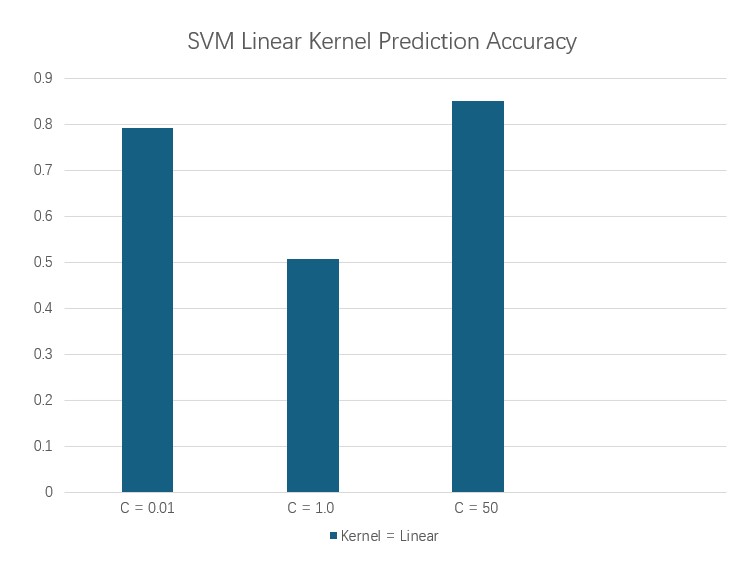
First, using a linear kernel SVM to predict midfielders’ performance. Here using three different values of C(they are 0.01, 1.0, and 50). This following confusin matrixes can evaluate the prediction performance of the linear kernel SVM model under different C vlaue. Accoridng to the formula of accuracy.

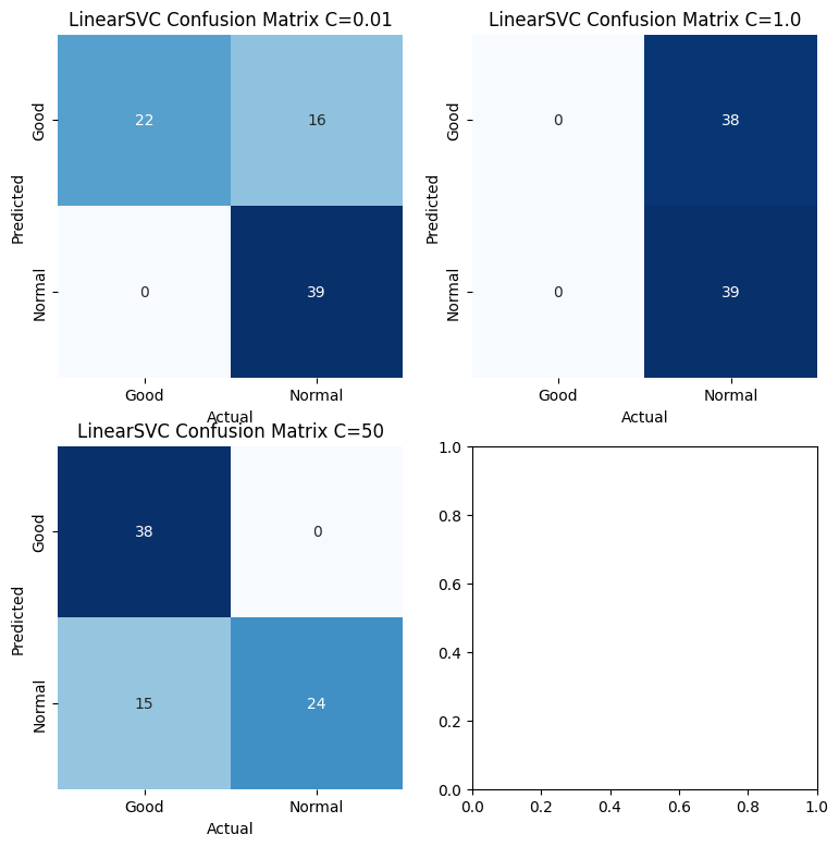
$$C_{0.01} = \frac{\text{Number of correlty classified Samples}}{\text{Total Number of Samples}} = \frac{22+39}{22+0+16+39} = 0.7922$$

$$C_{1.0} = \frac{\text{Number of correlty classified Samples}}{\text{Total Number of Samples}} = \frac{39}{38+39} = 0.5064$$

$$C_{50} = \frac{\text{Number of correlty classified Samples}}{\text{Total Number of Samples}} = \frac{38+24}{38+15+0+24} = 0.8052$$

prediction = svm_model.predict(playerTestDF_quant)
print(accuracy_score(playerTestLabel, prediction))

prediction2 = svm_model2.predict(playerTestDF_quant)
print(accuracy_score(playerTestLabel, prediction2))

prediction3 = svm_model3.predict(playerTestDF_quant)
print(accuracy_score(playerTestLabel, prediction3))

>>> 0.7922077922077922
>>> 0.5064935064935064
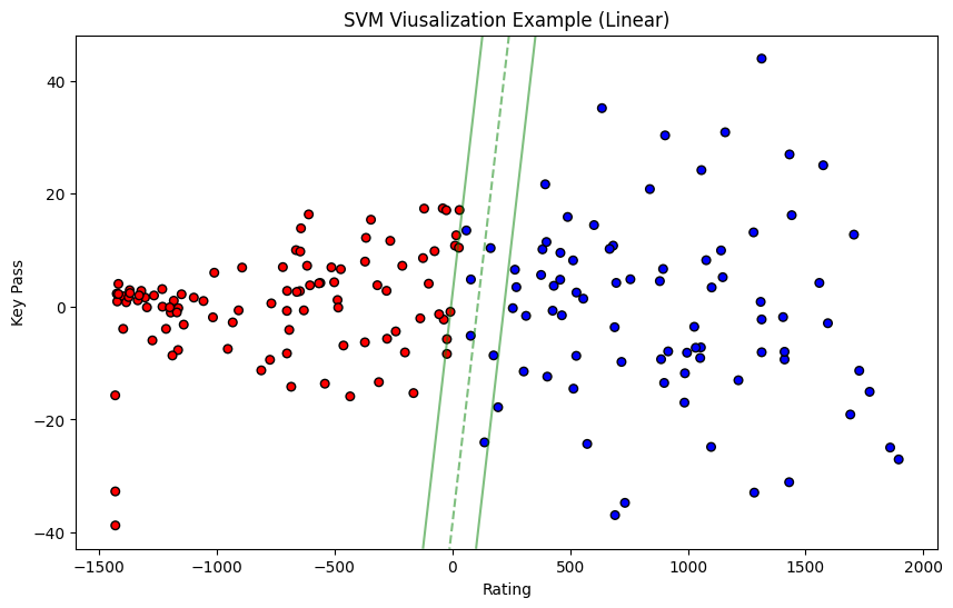
>>> 0.8051948051948052

From the accuracy of the prediction and confusion matrixes, the Linear SVM has a lower prediction accuracy of about 51% when C = 1.0. The accuracy of the model boosts to about 79% when C = 0.01. When C = 50, the model’s prediction accuracy is about 80%. Thus, the C value equal to 0.01 or 50 may be better than C = 1.0 when using the linear kernel. The following plot shows the visualization of the linear SVM model which the C value is 50.

Rbf Kernel

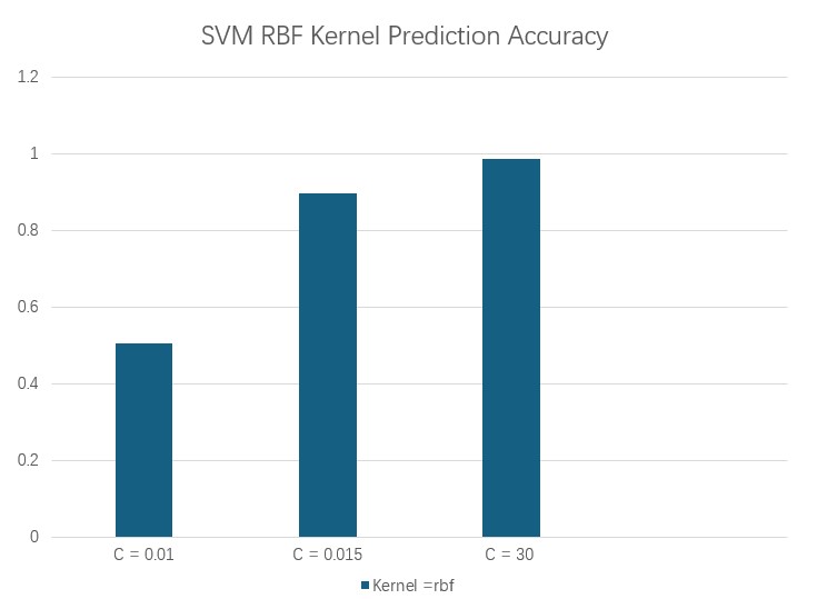
Using the rbf kernel SVM to predict midfielders’performance. Here using three diffierent value of C(they are 0.01, 0.015, and 30). This following confusion matrixes can evaluated the prediction performance of the rbf kernel SVM model under different C value. According to the formula of accuracy.

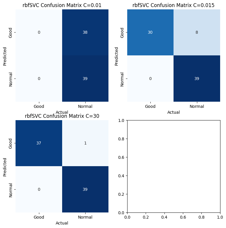
$$C_{0.01} = \frac{\text{Number of correlty classified Samples}}{\text{Total Number of Samples}} = \frac{39}{39+38} = 0.5064$$

$$C_{0.015} = \frac{\text{Number of correlty classified Samples}}{\text{Total Number of Samples}} = \frac{30+39}{30+8+39} = 0.8961$$

$$C_{30} = \frac{\text{Number of correlty classified Samples}}{\text{Total Number of Samples}} = \frac{37+39}{37+1+39} = 0.9870$$

rbf_prediction = svm_rbf_model.predict(playerTestDF_quant)
print(accuracy_score(playerTestLabel,rbf_prediction))

rbf_prediction2 = svm_rbf_model2.predict(playerTestDF_quant)
print(accuracy_score(playerTestLabel,rbf_prediction2))

rbf_prediction3 = svm_rbf_model3.predict(playerTestDF_quant)
print(accuracy_score(playerTestLabel,rbf_prediction3))

>>> 0.5064935064935064
>>> 0.8961038961038961
>>> 0.987012987012987

From the prediction accuracy and confusion matrixes of the rbf SVM model. It has a lower prediction accuracy of about 0.51% when C = 0.01. The accuracy of the model boosts to about 89.6% when C = 1.0. When C = 30, the model’s prediction accuracy is about 98.7%. Thus, the C value equal to 30 has better prediction affection than C equal to 1.0 and 0.01 when using the RBF kernel.

Polynomial Kernel

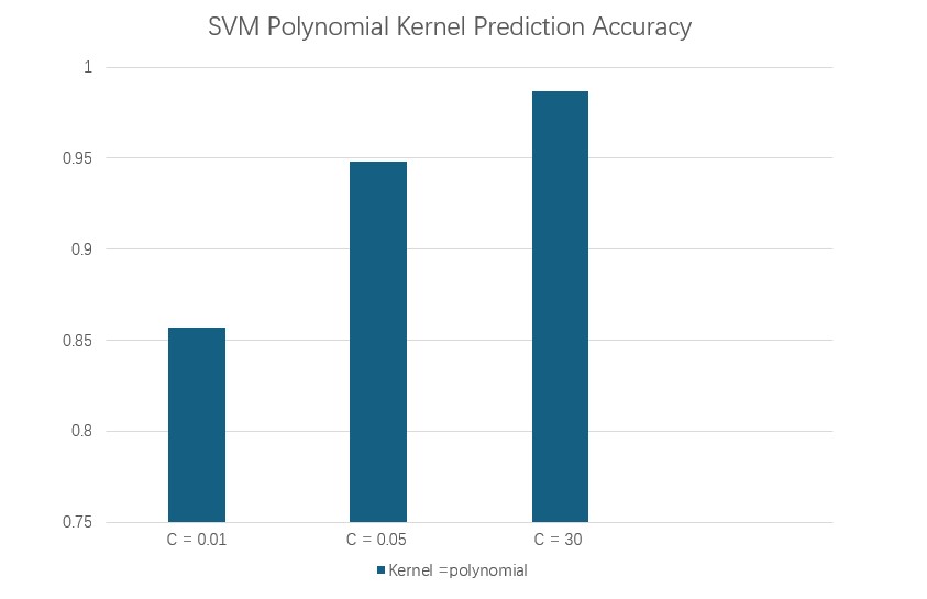
Using the polynomial kernel SVM to predict midfielders’ performance. Here using three different value of C(they are 0.01, 0.05, and 30). This following confusion matrixes can evaluated the prediction performance of the polynomial kernel SVM model under different C value. According to the formula of accuracy.

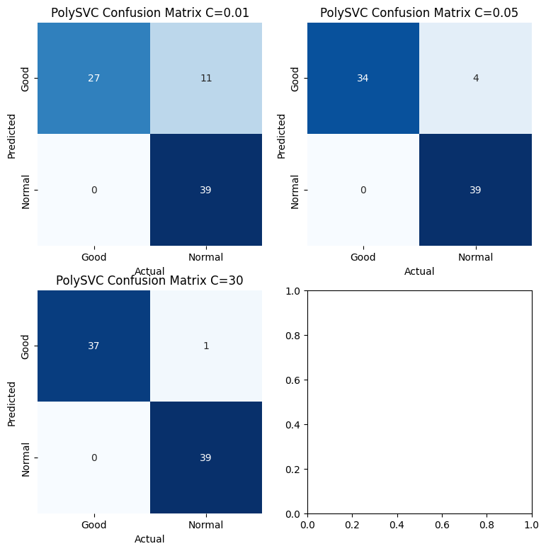
$$C_{0.01} = \frac{\text{Number of correlty classified Samples}}{\text{Total Number of Samples}} = \frac{27+39}{27+11+39} = 0.8571$$

$$C_{0.05} = \frac{\text{Number of correlty classified Samples}}{\text{Total Number of Samples}} = \frac{34+39}{34+4+39} = 0.9481$$

$$C_{30} = \frac{\text{Number of correlty classified Samples}}{\text{Total Number of Samples}} = \frac{37+39}{37+1+39} = 0.9870$$

poly_prediction = svm_poly_model.predict(playerTestDF_quant)
print(accuracy_score(playerTestLabel,poly_prediction))

poly_prediction2 = svm_poly_model2.predict(playerTestDF_quant)
print(accuracy_score(playerTestLabel,poly_prediction2))

poly_prediction3 = svm_poly_model3.predict(playerTestDF_quant)
print(accuracy_score(playerTestLabel,poly_prediction3))

>>> 0.857142857142857
>>> 0.948051948051948
>>> 0.987012987012987

From the prediction accuracy and confusion matrix of the polynomial SVM model. It has a lower prediction accuracy of about 85.7% when C = 0.01. The accuracy of the model improves to about 94.8% when C = 0.05. When C = 30, the model’s prediction accuracy is about 98.7%, Thus, the C value equal to 30 or 0.05 has better prediction affection than C equal to 0.01 when using the polynomial kernel.

Results

Comparing Different Kernels

The following bar plot shows the prediction accuracies using three different kernels(linear,rbf, and polynomial) at three different C values. It can be seen that linear kernel is slightly less effective than RBF and polynomial kernel during prediction processing. The prediction of the polynomial kernel function is the best among the three kernel functions. The prediction accuracy can reach more than 90% at different values of C. Therefore, selecting the polynomial kernel function using a C value of 50 is the final result of SVM prediction.

Prediction Result

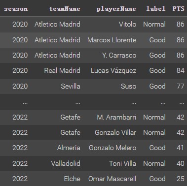
As a result, a club’s performance may depend on several midfielders performing well and working well together. For example, Atletico Madrid won the title in the 2020 season after stellar performances from midfielders such as Marcos Llorente and Carrasco managed to underpin the attacking and defensive transition throughout the entire season. On the contrary, if a team’s midfields lack good individual ability and good coordination, then the whole season may suffer such as Getafe. The midfielders such as Aranbarri and Gonzalo Vilar have normal performances, which caused Getafe to have a low ranking. Therefore, the performance of midfielders depends not only on their individual abilities but also on how well they correspond. These two key factors can have a significant impact on the trends of the clubs’ season.