Bayes Theorem
It is a theorem in probability theory that describes the probability that something will happen given some known conditions. For example, the duration of smoking is relatively high with lung cancer. Thus, using the formula of the Bayes theorem to accurately calculate how likely someone is to get lung cancer depending on their duration of smoking.
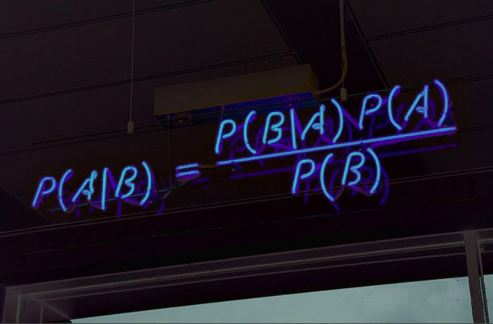
$$P(A | B) = \frac{P(A)P(B|A)}{P(B)}$$
$P(A | B)$: It is the posterior probability of A given the predictor B
$P(B | A)$: It is the likelihood, that probability of B given the A
$P(A)$: It is A Prior Probability that is probability of the A
$P(B)$: It is B prior Probability that is probability of the B
Here is an example that using the Bayes theorem
Doctors know that hyperthyroidism(H) causes a thick neck(T) is 60%, So $P(T|H) = 0.6$
Prior probability of any patient having hyperthyroidism is $\frac{1}{300}$, So $P(H) = \frac{1}{300}$
Prior probability of any patient having thick neck is $\frac{1}{60}$, So $P(T) = \frac{1}{60}$
The probability of a patient having hyperthyroidism if he/she has a thick neck.
$$P(H|T) = \frac{P(H)P(T|H)}{P(T)} = \frac{\frac{1}{300}*0.6}{\frac{1}{60}} = 0.12$$
Therefore, if a patient has a thick neck, he/she has the probability of hyperthyroidism is 12%.
Bayesian Classifiers
Bayes classifier is a class of classification algorithms based on Bayes theorem; Naïve Bayes classifier is one of them. It uses the Bayes theorem and calculates the posterior probability of each category based on the conditional probability of the input features, then selects the features with the highest posterior probability as the prediction results.
Naive Bayes Algorithm
The Naive Bayes algorithm is a machine learning classification algorithm based on Bayes theorem, and it is also a supervised learning algorithm. It will classify datasets by using Bayes’ theorem and the assumption of independence between features. In the real world, it is used for text classification, spam filtering, and sentiment analysis, etc.
There are serval variations of the Naive Bayes algorithm, such as Gaussian Naive Bayes, multinomial Naive Bayes, and Bernoulli Naive Bayes. These variations may apply to different types of features such as continuous, and discrete data types, and also apply to different distributions such as multinomial, gaussian, etc. Its advantage is that the simply implements the algorithm and is computationally efficient. It works well for high-dimensional data and large-scale datasets. But it assumes that the features are independent of each other, which is inconsistent in some cases in reality.
Multinomial Naive Bayes
Multinomial Naive Bayes is a kind of classification algorithm based on the Bayes theorem, and it is often used for text classification. It assumes that the probability distribution of the text sample is a multinomial distribution (Each feature is a discrete count value). These features could be words or phrases, and the value of each feature is the number of times the word or phrase appears in the text. In text classification, the text data needs to be converted into feature vectors at first, which can be represented by TF-IDF. Then, use a trained dataset to train a multinomial model to estimate the conditions probability distribution for each category. Finally, based on Bayes theorem, calculating the posterior probability of each category, and then picking a category with the greatest posterior probability as the final classification result.
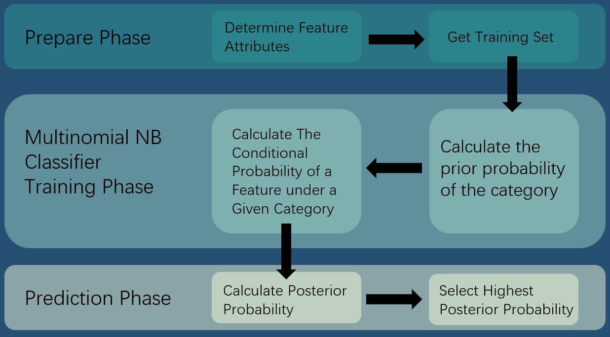
The process of text classification using Multinomial NB can be divided into two main steps (The figure shown below).
Training Phase
Count the number of documents for each category from the training dataset and calculate the prior probability of the category.
For each category, count the frequency of each feature under the category, and calculate the conditional probability of the feature under the given category.
Prediction Phase
For each category, calculate the posterior probability that the new documents belong to that category.
Select the category with the highest posterior probability as the prediction results.
Smoothing
Some features never appear in a category, which leads to a value of zero when calculating the condition probabilities. This situation may cause the model to be less predictive of never-before-seen features when predicted and may affect the model’s ability to generalize to new data. Thus, using the smoothing to deal with this issue. Common smoothing techniques such as Laplace smoothing and Lidstone smoothing. The main idea is to ensure the probability estimates for all features under each category are non-zero by adjusting the numerator and denominator of conditional probabilities. Smoothing is adding a small constant to the probability for each feature or adjusting the denominator to avoid it being zero. Therefore, using smoothing can prevent zero probability appear due to unseen features and improve the performance of the Multinomial NB model.
$$\text{Probability Estimation(Smoothing)}$$
$$\text{C:number of Classes, p: prior probability, m = parameter}$$
$$\text{Laplace:} P(A_i|C) = \frac{N_{iC}+1}{N_C + C}$$
$$\text{m-estimate:} P(A_i|C) = \frac{N_{iC}+mp}{N_C + m}$$
Bernoulli Naive Bayes
Bernoulli Naive Bayes is another variant of the Naive Bayes classifier and is mainly used to process binary data. It is also commonly used for text classification. It is different from multinomial Naive Bayes in that it mainly applies to binary features (the eigenvalues are usually 0 or 1). Therefore, the Bernoulli distribution is called a binary distribution, which means there are two possibilities for each event(Happen or not happen). It also needs to use smoothing techniques to handle features that do not appear in the training dataset to avoid the occurrence of 0 probabilities.
Plan For the Project
Analyzing the forwards(attackers) key capabilities of LaLiga, including passing accuracy, number of fouls, goal conversion rate, playing time, number of lines up, number of plays, number of key passes, and dribble success rate. And, using multinomial Naive Bayes to predict whether the summed ability of the forward players meets realistic expectations. Whether their overall ability is a key factor in a club’s ranking.