Decision Tree

Decision tree is a supervised learning algorithm for classification and regression tasks. It is a hierarchical tree mechanism that combines root nodes, branches, internal nodes, and leaf nodes.

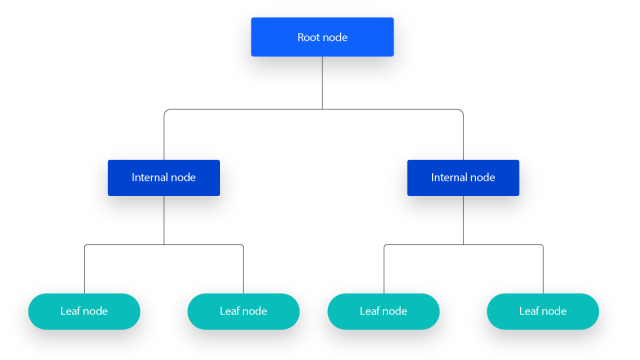
Root Node: It contains the whole set of samples.
Internal Nodes: It is corresponding feature attributes test
Leaf Nodes: It is decision results.

According to the figure shown below, this sample decision tree does not have any incoming branches from the root node, and then the branches from the root node start to provide information to the internal nodes (which are the decision nodes.). These two types of nodes both perform evaluations based on available functionality from a subset of the same class. The leaf nodes are these subsets and represent all possible decision outcomes.

Structure of Decision Tree

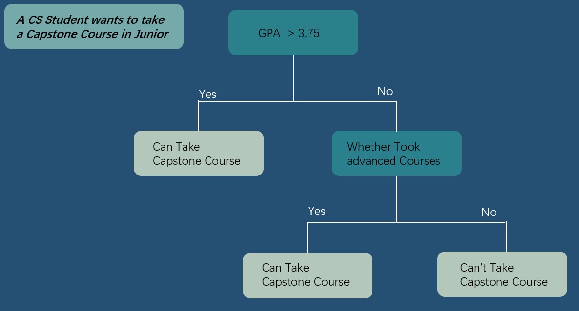
Hers is a simple example below, the CS department of a university to determine whether students can apply for the Capstone in their junior year. There are two indicators: GPA and whether students have taken advanced courses. From the figure blow, students with a GPA greater than 3.75 that can take Capstone course. If the students’ GPA are less than 3.75, it is necessary to determine whether the students had taken advance course. If they already did, they can. Otherwise, they cannot take the Capstone course.

Decision Tree Example

Steps for Decision Tree

Feature Selection: It determines which features do the judging. In the training dataset, each sample may have multiple attributes with different features playing a greater or lesser role. Thus, the function of feature selection is to pick the feature with a high correlation of classification results (The feature with strong classification ability). Some ways to select optimized feature such as Gini, Entropy, and Information Gain, and this part will be discussed later.
Decision Tree Generation: Assuming that using information gain is the most important feature selection criterion. Once the features are selected, the information gain of all the features is computed from all nodes. Then, the feature with the largest information gain is selected as a node and leaf nodes are created based on the different values of that feature. Using this method and so on until there is small information gain or no features to choose from.
Decision Tree Pruning: Its main purpose is to against overfitting, and it actively removes some branches to reduce the risk of overfitting.

Pros and Cons of Decision Tree

Advantage: It is easy to explain, and its Boolean logic and visualization help people to understand and use it. Also, the hierarchical structure of the decision tree makes it easier to spot essential features. It can handle discrete or continuous data types. It is also capable of handling data with missing values.

Disadvantage: Complex decision trees can overfit and do not work well with new data(decision tree pruning mentioned above can be avoided). Also, it is constructed using a greedy search method and its tanning cost will be higher than other algorithms.

Choosing The Best Way to Divide

The most important step in a decision tree is to choose an appropriate division way. Typically, as the division proceeds, the developers expect the branch nodes of the decision tree to contain samples that belong to the same category as much as possible to increase the purity of the nodes. For example, to identify the quality of seeds, the final expectation is to group good seeds with good seeds and bad seeds with bad seeds as much as possible. Information Gain (including Entropy) and Gini Impurity are commonly as segmentation metrics in decision trees, and they are used to evaluate the contribution of each test condition to classification and the ability to improve node purity.

Information Gain

Information gain is based on the change in entropy to determine the extent to which features contribute to the task of classification. The greater the information gain, the better classification results are obtained for feature division. Information entropy is the measure of uncertainty in datasets. Therefore, information gain is a measure of the effectiveness of features in reducing uncertainty and improving the purity of the datasets.

$$\text{Information Gain}(S,a) = \text{Entropy(S)} - \sum_{j=1}^{K}\frac{|S_j|}{|S|} \text{Entropy}(S_j)$$

$\text{a: Specific attributes or category label}$

$\text{S: Infomration Entropy of the dataset}$

$\sum_{j=1}^{K} \frac{|S_j|}{|S|} \text{Entropy}(S_j): \text{The conditional entropy of each feature}$

Information gain is a measure quantifies how much a given tree node split unmixes the labels at a node. Mathematically it is measure of the difference between impurity values before splitting the data at a node and the weighted average of the impurity after the split
source from: https://gatesboltonanalytics.com/?page_id=278

Entropy

Entropy is a metric used to measure the uncertainty of a dataset, the higher the entropy value, the higher the uncertainty of the dataset. This situation leads to a subset of a dataset containing a greater mix of different categories. Thus, during the division process, make sure that the lower the entropy value, which cases higher the purity of the divided subset.

$$\text{Entropy} = \sum_{i=1}^{C} - p_ilog_2(p_i) $$

$\text{S: Infomration entropy of dataset}$

$\text{C: categories in the set}$

$p_i:\text{Proportion of data points in category i to the total number of points in the dataset}$

Gini

Gini impurity is the probability of misclassification after classifying the data based on some feature. The lower the value of Gini, the more samples of the same category are included in the subset and the better affection of the division. If the dataset cannot be further divided, then its impurity is zero.

$$\text{Gini} = 1 - \sum_{i=1}^{C}{(p_i)^2}$$

During the processing of building a decision tree, using Gini as a picking feature method is a good way once encounter a dataset that contains a larger number of categorical categories, or to evaluate the nodes of the decision tree.

Example

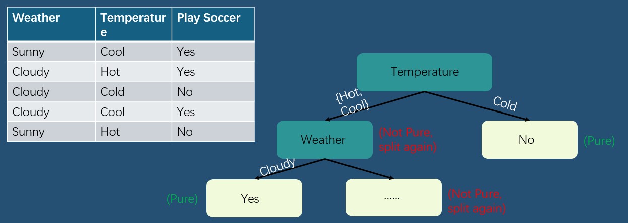
Dataset Sample

Entropy and Information Gain

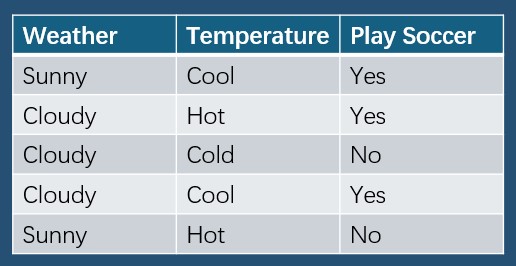
Calculate the entropy of origial dataset
$$P(\text{Play Soccer = Yes}) = \frac{3}{5} = 0.6 \text{, and } P(\text{Play Soccer = No}) = \frac{2}{5} = 0.4$$

$$ Entropy(S) = \sum_{i=1}^{C} - p_ilog_2(p_i) = -0.6log_2{0.6} - 0.4log_2{0.4} \approx 0.9710$$

Calcualte conditional entropy of Weather

$$P(\text{P= Yes | Weather = Sunny}) = \frac{1}{2} = 0.5 \text{, and } P(\text{P=No | Weather = Sunny}) = \frac{1}{2} = 0.5$$

$$P(\text{P=Yes | Weather = Cloud}) = \frac{2}{3} \text{, and } P(\text{P = No | Weather = Cloud}) = \frac{1}{3}$$

$$Entropy(S_\text{Sunny}) = \sum_{i=1}^{2} - p_ilog_2(p_i) = -0.5log_2{0.5} - 0.5log_2{0.5} = 1$$

$$Entropy(S_\text{Cloud}) = \sum_{i=1}^{2} - p_ilog_2(p_i) = -\frac{2}{3}log_2{\frac{2}{3}} - \frac{1}{3}log_2{\frac{1}{3}} = 0.9183$$

$$H(S|Weather) = \sum_{j=1}^{2}\frac{|S_\text{Weather}|}{|S|} \text{Entropy}(S_\text{Weather}) = \frac{2}{5} * 1+ \frac{3}{5} * 0.9183 = 0.9510$$

Calcuate the conditional entropy of Temperature

$$P(\text{P= Yes | Temp = Hot}) = \frac{1}{2} \text{, and } P(\text{P=No | Temp = Hot}) = \frac{1}{2}$$

$$P(\text{P=Yes | Temp = Cool}) = \frac{2}{2} \text{, and } P(\text{P = No | Temp = Cool}) = \frac{0}{2}$$

$$P(\text{P=Yes | Temp = Cold}) = \frac{0}{1} \text{, and } P(\text{P = No | Temp = Cold}) = \frac{1}{1}$$

$$Entropy(S_\text{Hot}) = \sum_{i=1}^{2} - p_ilog_2(p_i) = -0.5log_2{0.5} - 0.5log_2{0.5} = 1$$

$$Entropy(S_\text{Cool}) = \sum_{i=1}^{2} - p_ilog_2(p_i) = -\frac{2}{2}log_2{\frac{2}{2}} = 0$$

$$Entropy(S_\text{Cold}) = \sum_{i=1}^{2} - p_ilog_2(p_i) = -\frac{1}{1}log_2{\frac{1}{1}} = 0$$

$$H(S|Temp) = \sum_{j=1}^{2}\frac{|S_\text{Temp}|}{|S|} \text{Entropy}(S_\text{Temp}) = \frac{2}{5} * 1+ \frac{2}{5} * 0 + \frac{1}{5}*0 = 0.4$$

Calcuate the information gain for each feature

$$\text{Information Gain}(S,Weather) = \text{Entropy(S)} - \sum_{j=1}^{K}\frac{|S_j|}{|S|} \text{Entropy}(S_j) = 0.9710 - 0.9510 = 0.02$$

$$\text{Information Gain}(S,Temp) = \text{Entropy(S)} - \sum_{j=1}^{K}\frac{|S_j|}{|S|} \text{Entropy}(S_j) = 0.9710 - 0.4 = 0.571$$

Therefore, choosing feature of Temperature as the first split point, because $\text{Information Gain}(S,Temp) > \text{Information Gain}(S,Weather)$

Demo for Splitting Process

Create an infinite number of trees

In each split of a node, the decision tree can select the best-split point from multiple features. Also, the continuity features are able to choose different division points, so this allows the decision tree to create many different topologies. Second, for large-scale datasets with many features, a decision tree may create deeper trees to better fit the data. It can be able to classify or regress the data better.

Plan For the Project

Analyzing the defenders key capabilities of LaLiga, including tackle blocks, tackle interception, and fouls committed. Using decision tree algorithms to predict whether the summed ability of the defensive players meets realistic expectations. Whether their overall ability is a key factor in a club’s ranking.