Accuracy of Decision Trees Prediction
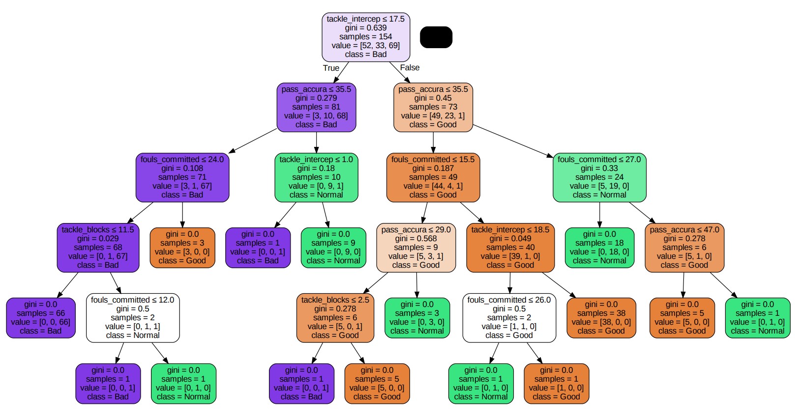
Decision Tree Model 1 : Gini & Better Splitter
In the first model, the main changed parameters are criterion=gini and splitter=better. Here, splitter=better means the best splitting method. At each tree node, the algorithm tries all combinations of features and eigenvalues. Then it selects the segmentation that allows the most improvement in the purity of the leaf nodes. The final tree plot is shown below.
This following confusion matrix can evaluate the prediction preformance of this model. According to the fomula of accuracy.
$$\frac{\text{Number of corretly classified Samples}}{\text{Total Number of Samples}} = \frac{19+13+25}{19+4+0+1+13+2+3+0+25} \approx 0.85$$
from sklearn.metrics import accuracy_score
accuracy = accuracy_score(playerTestLabel, predictions)
print(accuracy)

>>> 0.8507462686567164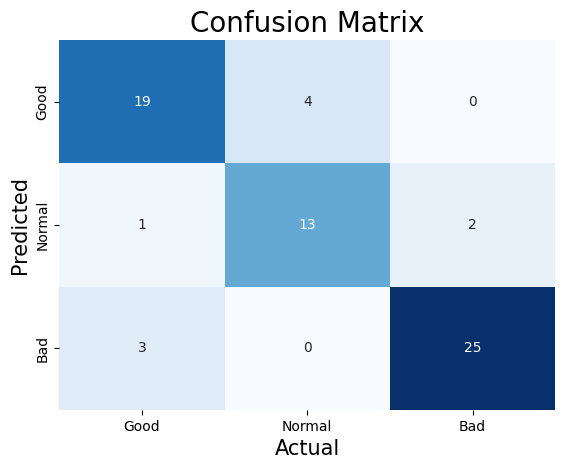
Therefore, this model is about 85% accurate in predicting categories. And getting the precision rate for each category by using the confusion matrix:
$$\text{‘Good’ Precision} = \frac{19}{19+1+3} \approx 0.83$$
$$\text{‘Normal’ Precision} = \frac{13}{4+13+0} \approx 0.77$$
$$\text{‘Bad’ Precision} = \frac{25}{0+2+25} \approx 0.93$$
Based on these precision rates can be seen that category of Bad has highest precision rate, which is about 93%. The category of Normal has lowest precision rate of about 77%. Thus, predicting the category as Bad is the most accurate, and predicting the category as Normal is less effective than other two categories.
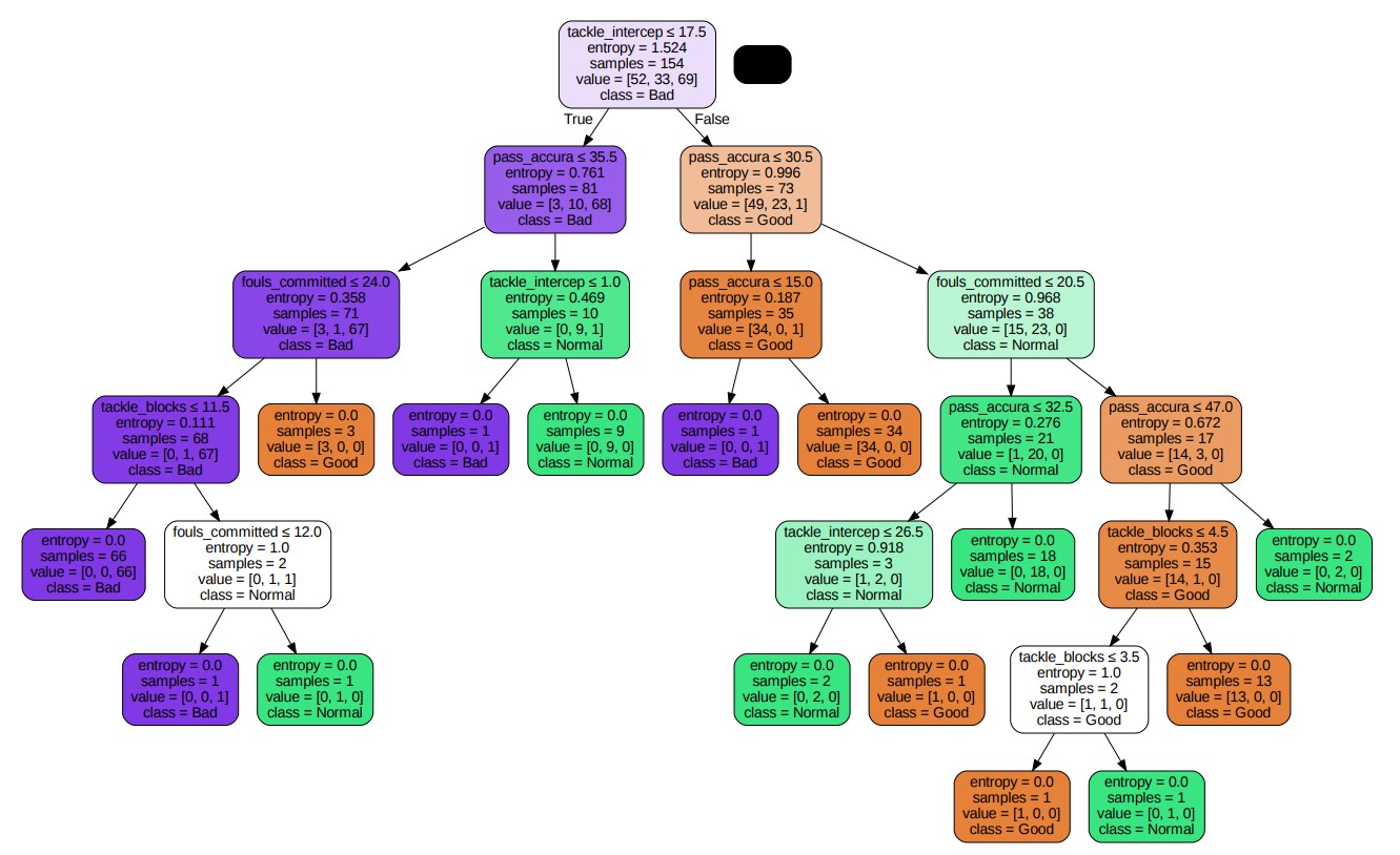
Decision Tree Model 2: Entropy & Better Splitter
In the second model, the main changed parameter is criterion=Entropy The second tree plot is shown below.
This following confusion matrix can evaluate the prediction preformance of this model. According to the fomula of accuracy.
$$\frac{\text{Number of corretly classified Samples}}{\text{Total Number of Samples}} = \frac{21+9+25}{21+2+0+5+9+2+3+0+25} \approx 0.82$$
from sklearn.metrics import accuracy_score
accuracy2 = accuracy_score(playerTestLabel, predictions2)
print(accuracy2)

>>> 0.8208955223880597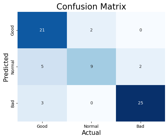
Therefore, this model is about 82% accurate in predicting categories. And getting the precision rate for each category by using the confusion matrix:
$$\text{‘Good’ Precision} = \frac{21}{21+5+3} \approx 0.72$$
$$\text{‘Normal’ Precision} = \frac{9}{2+9+0} \approx 0.81$$
$$\text{‘Bad’ Precision} = \frac{25}{0+2+25} \approx 0.93$$
Thus, according to these precision rates can be seen that category of Bad has highest precision rate, which is about 93%. The category of Good has lowest precision rate of about 77%. Thus, predicting the category as Bad is the most accurate, and predicting the category as Good is less effective than other two categories.
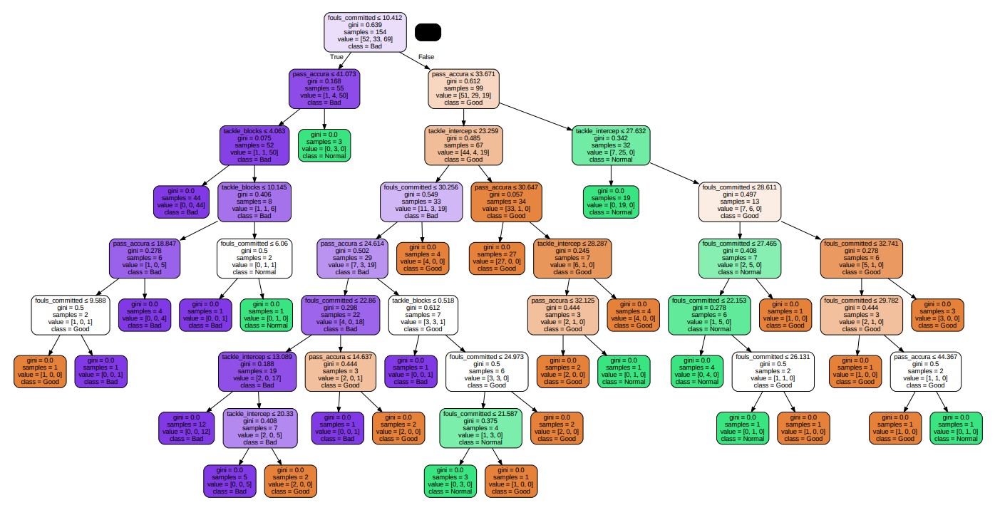
Decision Tree Model 3: Gini & Random Splitter
In the third model, the main changed parameter is splitter=random. Here, splitter=random means the best splitting method. At each tree node, the algorithm random select a feature and a eigenvalue. It leads to greater randomness in the generated decision tree. The third tree plot is shown below.
This following confusion matrix can evaluate the prediction preformance of this model. According to the fomula of accuracy.
$$\frac{\text{Number of corretly classified Samples}}{\text{Total Number of Samples}} = \frac{20+16+25}{20+3+0+0+16+0+3+0+25} \approx 0.91$$
from sklearn.metrics import accuracy_score
accuracy3 = accuracy_score(playerTestLabel, predictions3)
print(accuracy3)

>>> 0.9104477611940298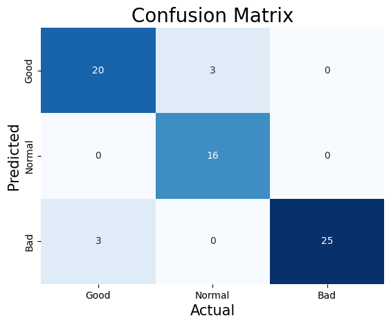
Therefore, this model is about 91% accurate in predicting categories. And getting the precision rate for each category by using the confusion matrix:
$$\text{‘Good’ Precision} = \frac{20}{20+0+3} \approx 0.87$$
$$\text{‘Normal’ Precision} = \frac{16}{3+16+0} \approx 0.84$$
$$\text{‘Bad’ Precision} = \frac{25}{0+0+25} \approx 1.00$$
Therefore, according to these precision rates can be seen that category of Bad has highest precision rate, which is about 100%. The category of Normal has lowest precision rate of about 84%. Thus, predicting the category as Bad is the most accurate, and predicting the category as Normal is less effective than other two categories.
Result
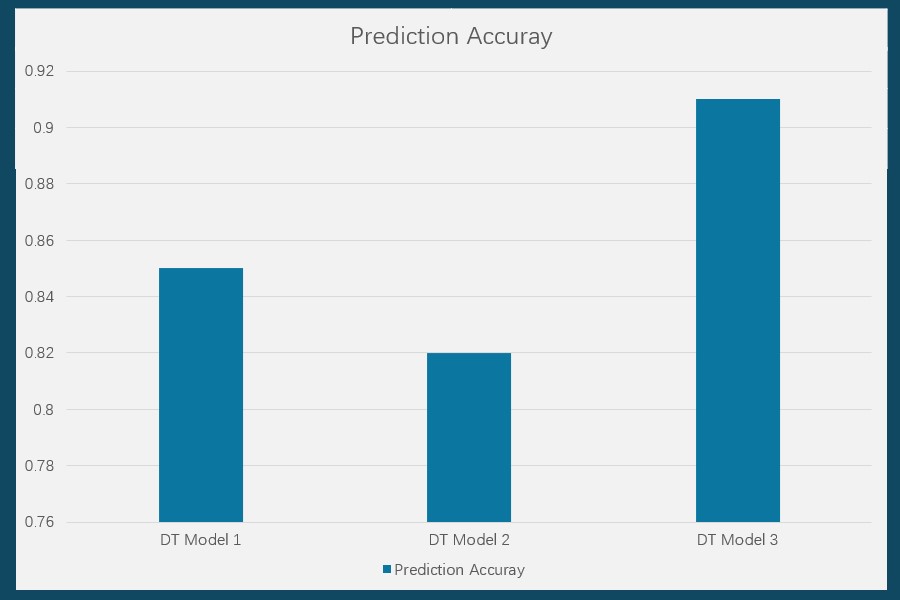
From the bar plot, the model 3 has the best prediction affection in the decision tree models. It is about 91% accurate. Using this model to show performance prediction for defenders (show shown below).
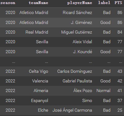
The model’s predictions are good. For example, Sevilla defender J.Kounde. During the 2020 season, he was in great form and attracted the attention of Chelsea and FC Barcelona. Eventually, he chose to join Barcelona. At FC Barcelona, he was highly regarded and won the La Liga title for the club. Also, Atletico Madrid defender J.Gimenez shined in the 2020 season, winning the La Liga title for his club in 2020. Therefore, these predictions are realistic.